Identification and Visualization of Variability Implementations in Object-Oriented Variability-Rich Systems: A Symmetry-Based Approach
Useful links
symfinder’s source code
The source code of symfinder is available here (tag: jrn20).
Generated visualizations
The output visualizations of symfinder for the 16 projects are deployed here.
Ground truths
Here are the ground truths used for the mappings in ArgoUML and Sat4j. They contain the trace links of the domain features to their respective code assets.
ArgoUML’s ground truth is available here.
Sat4j’s ground truth is available here.
Mapping process
Details on the mapping process are available here.
symfinder’s artifacts
Current public release
The latest publicly released source code of the symfinder tool, tagged jrn20, is available for download at https://github.com/DeathStar3/symfinder.
symfinder usage guidelines
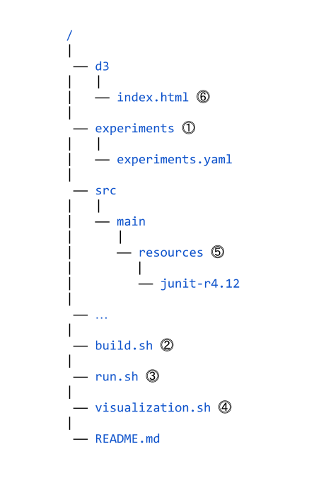
Here is the main project structure of symfinder.

The numbers on the right side show the sequence of steps to reproduce any of the presented experiments.
The README.md file contains a detailed guide on the technical requirements, how to set up an experiment, to run it, and how to visualize the resulting data for analysis.
This guide is valid for three operating systems, GNU/Linux, macOS Sierra 10.12 or newer, and Windows 10 64-bit (Pro, Enterprise or Education).
The main requirements for the toolchain are Docker and Docker Compose, so to facilitate the overall portability.
The experiments.yaml file in ⓵ is used to set up an experiment.
It requires the git repository url of the targeted system with its tag ID or commit ID, for instance, the url of JUnit with tag r4.12.
The provided file contains a default configuration that corresponds to all first sixteen analysed systems listed in the paper.
Still, one can change the configuration to analyse another set of systems.
In ⓶ and ⓷, build.sh and run.sh are the main scripts to build and run an experiment.
Basically, run.sh downloads the sources of the targeted system and starts a Docker Compose environment, whereas visualization.sh in ⓸ generates the visualization data.
The downloaded copy of a system is saved locally in the resources folder, such as the junit-r4.12 subfolder in ⓹.
Then, index.html is used to access the generated visualization of the identified variability for a targeted system (⓺). It can be opened locally using a web browser, through http://localhost:8181.
The README.md file also contains a visualization example, which is annotated to explain the different elements of visualization.
symfinder’s identification method
symfinder relies on a Neo4j database to identify the symmetries. The Cypher requests used to query the database are listed here.